How to tackle overfitting via regularization in machine learning models

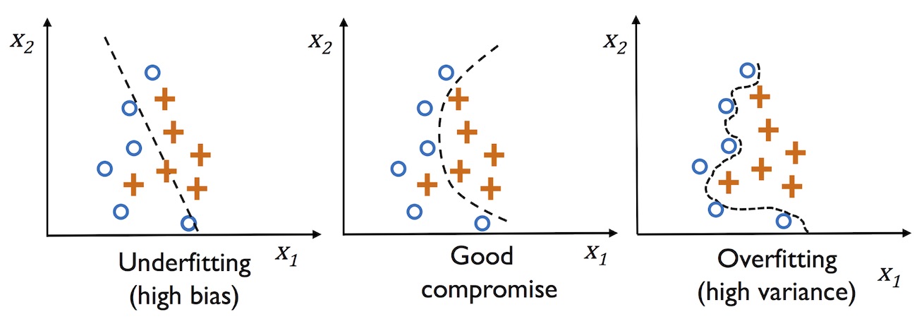
Overfitting is a common problem in machine learning, where a model performs well on training data but does not generalize well to unseen data (test data). If a model suffers from overfitting, we also say that the model has a high variance, which can be caused by having too many parameters, leading to a model that is too complex given the underlying data. Similarly, our model can also suffer from underfitting (high bias), which means that our model is not complex enough to capture the pattern in the training data well and therefore also suffers from low performance on unseen data.

This article is an excerpt from the book Python Machine Learning, Third Edition by Sebastian Raschka and Vahid Mirjalili. This book is updated for TensorFlow 2 and the latest additions to scikit-learn. This new third edition of the book is now available at 20% off now (offer is valid till 8th September 2020).

The problems of overfitting and underfitting can be best illustrated by comparing a linear decision boundary to more complex, nonlinear decision boundaries, as shown in the following figure:

The bias-variance tradeoff

Often, researchers use the terms “bias” and “variance” or “biasvariance tradeoff” to describe the performance of a model—that is, you may stumble upon talks, books, or articles where people say that a model has a “high variance” or “high bias.” So, what does that mean? In general, we might say that “high variance” is proportional to overfitting and “high bias” is proportional to underfitting.

In the context of machine learning models, variance measures the consistency (or variability) of the model prediction for classifying a particular example if we retrain the model multiple times, for example, on different subsets of the training dataset. We can say that the model is sensitive to the randomness in the training data. In contrast, bias measures how far off the predictions are from the correct values in general if we rebuild the model multiple times on different training datasets; bias is the measure of the systematic error that is not due to randomness.

One way of finding a good bias-variance tradeoff is to tune the complexity of the model via regularization. Regularization is a very useful method for handling collinearity (high correlation among features), filtering out noise from data, and eventually preventing overfitting.

Tackling overfitting via regularization

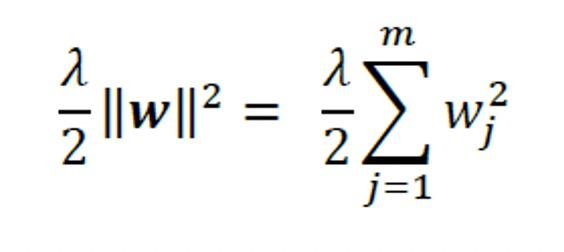
The concept behind regularization is to introduce additional information (bias) to penalize extreme parameter (weight) values. The most common form of regularization is so-called L2 regularization (sometimes also called L2 shrinkage or weight decay), which can be written as follows:

Here, 𝜆 is the so-called regularization parameter.

Note: Regularization is another reason why feature scaling such as standardization is important. For regularization to work properly, we need to ensure that all our features are on comparable scales.

The cost function for logistic regression can be regularized by adding a simple regularization term, which will shrink the weights during model training:

Via the regularization parameter, 𝜆, we can then control how well we fit the training

data, while keeping the weights small. By increasing the value of 𝜆, we increase the regularization strength.

The parameter, C, that is implemented for the LogisticRegression class in scikitlearn

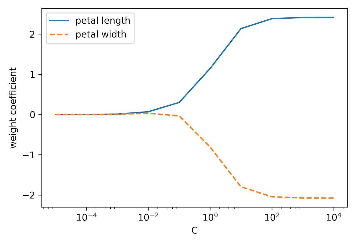
comes from a convention in support vector machines. The term C is directly related to the regularization parameter, 𝜆, which is its inverse. Consequently, decreasing the value of the inverse regularization parameter, C, means that we are increasing the regularization strength, which we can visualize by plotting the L2 regularization path for the two weight coefficients:

>>> weights, params = [], []

>>> for c in np.arange(-5, 5):

…     lr = LogisticRegression(C=10.**c, random_state=1,

…                             solver=’lbfgs’, multi_class=’ovr’)

…     lr.fit(X_train_std, y_train)

…     weights.append(lr.coef_[1])

…     params.append(10.**c)

>>> weights = np.array(weights)

>>> plt.plot(params, weights[:, 0],

…          label=’petal length’)

>>> plt.plot(params, weights[:, 1], linestyle=’–‘,

…          label=’petal width’)

>>> plt.ylabel(‘weight coefficient’)

>>> plt.xlabel(‘C’)

>>> plt.legend(loc=’upper left’)

>>> plt.xscale(‘log’)

>>> plt.show()

By executing the preceding code, we fitted 10 logistic regression models with different values for the inverse-regularization parameter, C. For the purposes of illustration, we only collected the weight coefficients of class 1 (here, the second class in the dataset: Iris-versicolor) versus all classifiers—remember that we are using the OvR technique for multiclass classification.

As we can see in the resulting plot, the weight coefficients shrink if we decrease parameter C, that is, if we increase the regularization strength:

In this article, you learned about a machine learning algorithm that is used to tackle the overfitting problems. Python Machine Learning, Third Edition is a comprehensive guide to machine learning and deep learning with Python, scikit-learn, and TensorFlow 2 with a coverage on GANs and reinforcement learning.

About the Authors

Sebastian Raschka is an Assistant Professor of Statistics at the University of Wisconsin-Madison focusing on machine learning and deep learning research. Some of his recent research methods have been applied to solving problems in the field of biometrics for imparting privacy to face images. Other research focus areas include the development of methods related to model evaluation in machine learning, deep learning for ordinal targets, and applications of machine learning to computational biology. Vahid Mirjalili obtained his Ph.D. in mechanical engineering working on novel methods for large-scale, computational simulations of molecular structures. Currently, he is focusing his research efforts on applications of machine learning in various computer vision projects at the Department of Computer Science and Engineering at Michigan State University. He recently joined 3M Company as a research scientist, where he uses his expertise and applies state-of-the-art machine learning and deep learning techniques to solve real-world problems in various applications to make life better.